FluidFlow3 is the first and only integrated software for piping system design, calculation and optimization that supports liquids, gases, slurries, 2-phase, and non-Newtonian fluids. FluidFlow3 is a truly original software program for the complete hydraulic design, network analysis, trouble-shooting and optimization of piping systems. The solution include flows, pressures, temperatures and phase states through out your piping network.

FluidFlow3 means efficient and accurate modeling for the design of energy efficient, safe reliable flow systems that are easy to operate and maintain. A wide variety of industries depend on FluidFlow3 to successfully model new and existing systems, size pipes, select boosters, controllers and other fluid equipment.

All modules have, as standard, the ability to include heat loss/gain from pipes. Temperature or heat transfer to or from equipment is also included.

Product Modules

Liquids, Incompressible Fluid Flow
Gas, Compressible Flow
Two Phase Liquid-Gas Flow
Settling Slurries
Non-Newtonian, Non-Settling Slurry Flow
Heat Transfer
Dynamic Analysis & Scripting

__________________________________________________________________________________________________________________

Liquids, Incompressible Fluid Flow

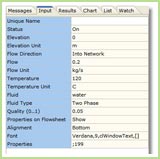
Engineers using FluidFlow3 can determine the pressure, flow, temperature, and phase state at any point within their pipe systems. Any type and any size of piping system can be modelled. Real piping systems often contain many different types of components and fittings.

FluidFlow3 can model any component (fluid equipment item) you are likely to come across, these include: boosters (positive displacement and centrifugal types), valves (including 3-way), flow controllers, pressure sustainers, pressure reducers, differential pressure controllers, check and non return valves, orifice plates, reducers & expanders, venturi tubes, inline nozzles, filters, packed beds, cyclones, centrifuges, labyrinth seals, pipe coils, relief valves, bursting disks, shell & tube exchangers, plate exchangers, auto-claves, knock-out pots, as well as rigorously modelling junctions (tees, wyes, bends, & crosses). For items not covered by the above you can define your own.

For liquid (incompressible flow) calculations, FluidFlow3 solves the fundamental conservation equations of mass, energy, and momentum. Solution of the energy and momentum equations for an incompressible fluid results in:

• Darcy Weisbach equation
• Bernoulli's principle

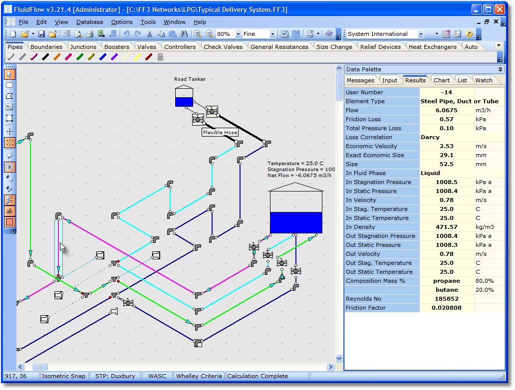
Liquid modelling of a LNG storage delivery system

The example opposite shows the main take off line for tanker loading from a LNG storage tank facility.

FluidFlow3 solves continuity, momentum and energy equations iteratively to arrive at an accurate solution. Phase states and physical properties are estimated at each point in the network. Solutions are valid for all flow regimes.

As well as modelling the liquid lines, FluidFlow3 can also model the vapor lines to the external compressor.

Gas, Compressible Flow

When a gas flows in a pipe network the gas density, temperature and velocity change as the fluid flows through the network.

A solution approach often used in the literature is to assume ideal gas laws so that analytical equations for energy, momentum and continuity equations can be derived. Rather than make these simplifying assumptions FluidFlow3 uses a calculation procedure that solves the conservation equations together with an equation of state for small pressure loss increments. This means FluidFlow3 obtains a rigorous solution.

Available equations of state are:

• Benedict-Webb-Rubin
• Peng-Robinson
• Lee Kesler

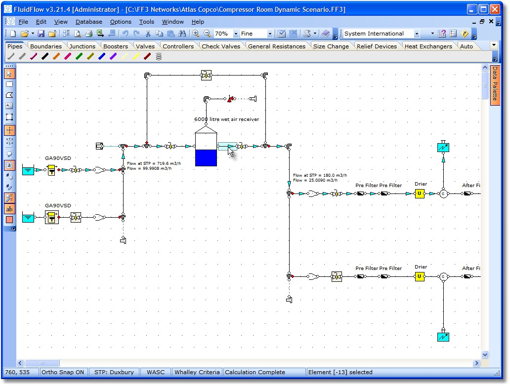
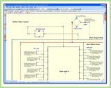
Compressor Room Dynamic Scenario

The example opposite shows an air compression and receiver system.

PD Compressors, Air Filters, Recievers, Driers & Relief Systems can all be included in the same model.

Dynamic scenarios are best considered using script, but of course alternate design scenarios can be considered via the Input Editing facilities available with all versions and modules.

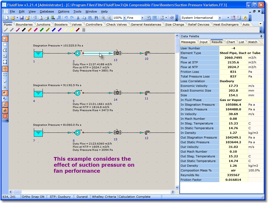
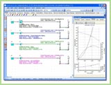
Gas Results

Consider the tabular results for the fan discharge pipe as shown opposite. Along the flowpath the gas expands, the temperature and density decreases, while the velocity and actual flow increases. This is the case if no heat transfer occurs, FluidFlow3 can also take heat transfer considerations into account.

You may also notice that we are displaying 3 volumetric flows in the results table. The first flow refers to the actual flow at the start of the pipe (remember the actual volumetric flow increases as gas flows down the pipe), the other flow rates show volumetric flow with reference to standard and normal conditions.

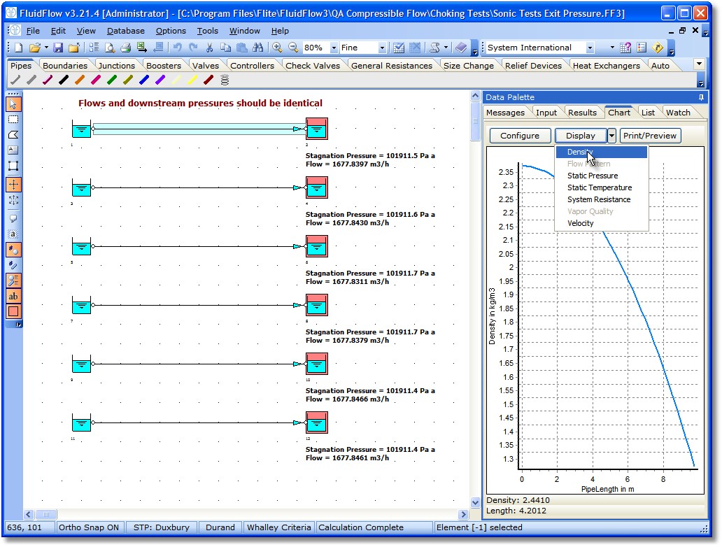
Gas Chart Results

For gas flow within a pipe, the pressure and temperature conditions continuously change. This means that the gas physical properties of density, viscosity, heat capacity, thermal conductivity, sonic velocity, etc., change with pipe length.

The curve opposite shows the change in gas density as we flow down this pipe. This underlines the importance of using an appropriate calculation method. Imagine the error that would be introduced if you assumed density was constant.

Two Phase Liquid-Gas Flow

The two phase flow module allows two phase liquid-gas calculations to be accomplished. Two phase flow occurs in many industrial processes. Examples are petroleum, chemical, nuclear, refrigeration, space, and geothermal industries.

FluidFlow3 can analyse systems where the vapor quality changes with pipe position as well as two phase flow where the vapor quality is fixed.

FluidFlow3 uses a modelling approach for the pressure loss calculation, this is a hybrid between the rigorous and empirical methods. By this, we mean, that we use well known empirical correlations and apply them to a differential pipe length. This allows for a flash calculation, liquid holdup and flow regime to be determined for each segment and acknowledges that the pressure loss per unit length changes as the two phase mixture flows down the pipe.

The available pressure loss relationships that you can use in FluidFlow3 are:

• Friedel: This method is based on the paper published by Friedel and utilises a two phase multiplier to the liquid pressure loss calculation.
• Chisholm: Proposed an extensive empirical method (1973), which also uses a two phase multiplier.
• Lockhart-Martinelli: Proposed a separated flow model, but this should only be applied to horizontal flow.
  
  Comparison of the above 3 methods to a recent two phase database was made by Whalley who made the following recommendations:(µL/µG) < 1000 and a mass flux of < 2000 kg/m2s use the Friedel method.

(µL/µG) > 1000 and a mass flux of > 100 kg/m2s use the Chisholm method.

(µL/µG) > 1000 and a mass flux of < 100 kg/m2s use the Lockhart Martinelli method.

If you select the Whalley Criteria in the Calculation Options dialog. FluidFlow3 will select the appropriate method for you.

• More recently Muller Steinhagen and Heck (2000) made an updated comparison and recommended the MSH correlation as a better approach, particularly for refrigerants and single component fluids. This method looses accuracy at high vapor quality.
• One of the first approaches based on flow regime was made by Beggs Brill. This correlation is applicable to all pipe orientations. The original method (1973) was extended and FluidFlow3 uses the extended method. You should probably not use this method for vertical upflow because it underpredicts pressure loss.
• Drift Flux modelling is accommodated in FluidFlow3 by using a new correlation published in 2007 [22], this model is best suited for vertical and inclined pipes.

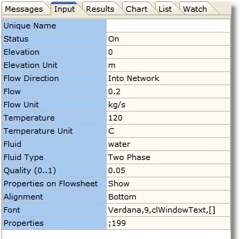
Two phase input data

The example opposite shows the Input Editor defined for the supply of a two phase mixture of steam and water fed directly into a network.

FluidFlow3 will calculate the change in vapor quality as the two phase mixture flows down the pipe.

FluidFlow3 also allows multiphase mixtures to be made via the flowsheet.

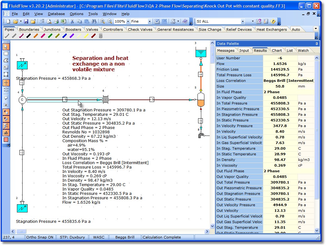
Two fluids mixed on a flowsheet

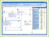
The flowsheet shows two known flows (one fluid air(2), one fluid water(1)) combining and being heated via a plate exchanger, then flowing to a separation vessel (5). The red dot on the Knock Out Pot (separator) represents the liquid outlet and the yellow dot represents the vapor outlet.

This is an example of two phase flow with constant quality. This means that the vapor mass fraction is constant and there is no mass transfer between the phases. It does not mean that the pressure loss per unit length is constant or that the velocity between the two phases is constant. In the first pipe section after mixing (pipe -6) you can see that the gas superficial velocity increases from the start to the end of pipe -6. For 60m of pipe -6, the total pressure loss is 145997 Pa, but the friction loss is 144529 Pa. Since the pipe is horizontal the difference is the acceleration loss.

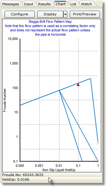
Pipeline flow pattern map for two phase flow

The horizontal flow pattern map for the Beggs and Brill method is shown opposite. This correlation is applicable to the entire range of pipe inclination angles, although it usually underpredicts pressure loss for vertical upward flow.

In this example the predicted flow pattern is in the intermittant region.

Using a mechanistic modelling approach a more accurate model of the flow pattern map can be achieved.

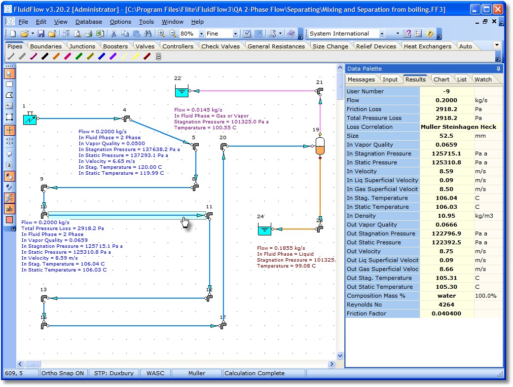
Separation from a boiling mixture

This example shows a boiling mixture of steam and water flowing through a pipe network to a vapor-liquid separator. The calculated results have been exported to Excel. The content of the export can be controlled.

You can download the xls file produced by FluidFlow3 by clicking here.

Settling Slurries

Settling slurries comprise a carrier fluid conveying solid particles. This type of flow has extensive applications in the mining and mineral processing industries, where the design of pumped systems must take into account the effect of solids on pipe friction loss and pump performance.

Simulating the performance of settling slurries is dependant on the solid density, concentration, particle shape and size distribution, as well as the properties of the carrier fluid. Selecting the optimum pipeline velocity is usually the most important factor in the design and operation of slurry systems. Operating with velocities too high wastes energy, while operating with velocities too low can lead to pipeline blackage.

Design methods are highly empirical and FluidFlow3 offers different calculation approaches:

• Wilson-Addie-Sellgren-Clift (WASC)
• Durand-Condolios-Worster
• WASP

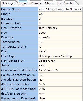
Carrier and solids input data

The example opposite shows the Input Editor defined for the transportation of 1000 tonne/h of sand at a volume concentration of 30%.

FluidFlow3 will calculate the correct volumetric flowrate to acheive this requirement. We could have specified flow as total volumetric, or on a carrier basis only.

Particle size entry requirements depends on the calculation approach selected. WASC requires d50 and d85, Durand requires d50 and WASP requires a particle size distribution which the software allows.

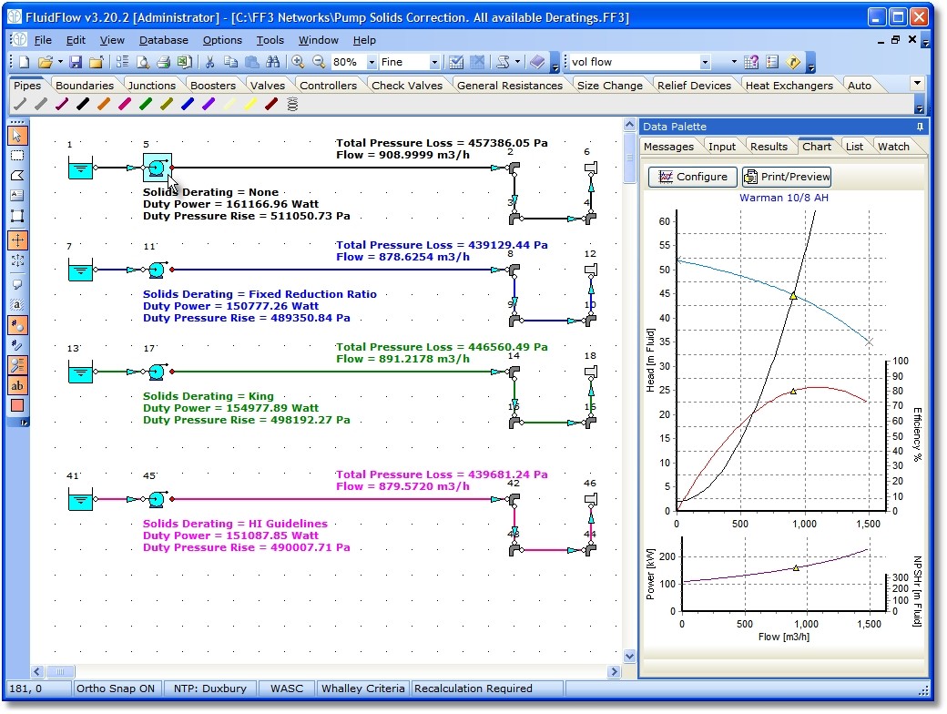
Pump Deration

When a pump is used to transport a slurry, the prescence of the solid particles has a significant effect on the performance of the pump. As the concentration of slurry increases, the head generated by the pump decreases because of the greater friction losses that occur in the pump casing.

FluidFlow3 allows you to select the amount of derating that is applied. This value may be obtained from the pump supplier, or FluidFlow3 can estimate the deration according to Hydraulic Institude guidelines or via other text book calculation methods.

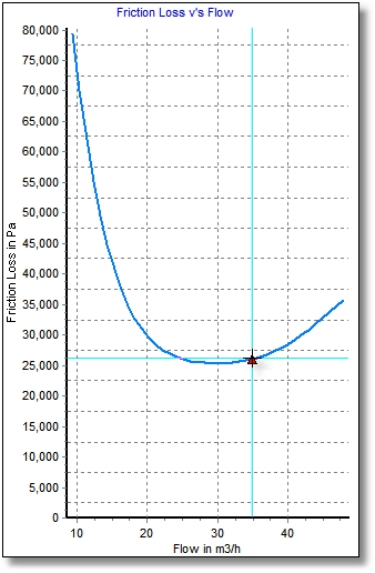
Pipeline system curve for a settling slurry

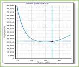
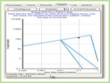
The system curve for a settling slurry is different to that of a Newtonian fluid. The friction loss curve for a nickle ore slurry is shown opposite. A minimum friction loss value is usually observed at or near the particle deposit velocity. The most economical velocity is usually at this minimum point.

The curve shown is asymptotic to the equivalent water curve at higher velocities, so essentially the slurry flow calculations are calculations of the "solids effect" of the suspended solids, i.e., the additional pressure loss due to the suspended solids over that for the same volumetric flow of the carrier alone.

Usually, because of the application of safety factors in design methods, pipelines are operated at higher flow velocities than the economic minimum. There are a series of system curves, the exact position and shape of each curve depends on the solid concentration.

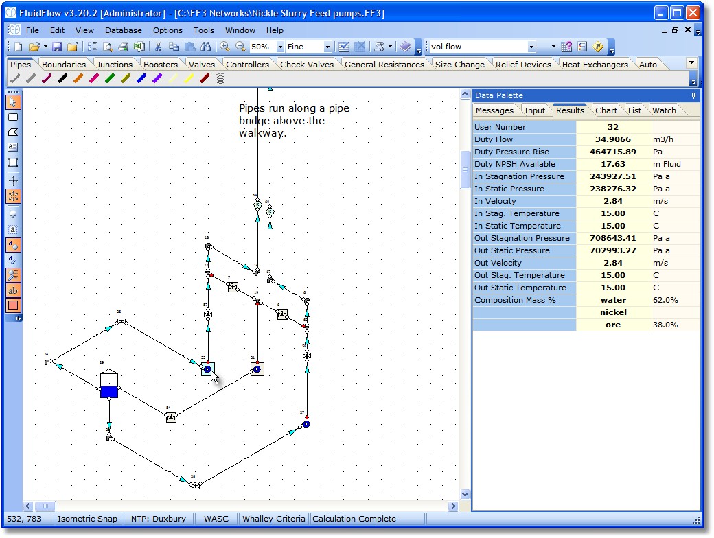
Nickle ore delivery system

This example shows a pumped slurry system that has been exported to Excel. The content of the export can be fully controlled.

You can download the xls file produced by FluidFlow3 by clicking here.

Click on the tabs to display the various Excel pages. Exporting to Excel allows you to customise your reports and provides an excellent method of communicating the results of a study, to a client or colleague.

Non-Newtonian, Non-Settling Slurry Flow

A non-Newtonian fluid is a liquid whose flow properties are not described by a single constant value of viscosity. Examples of non-Newtonian fluids are: polymer solutions, starch suspensions, paint, blood, food products, and mining suspensions of densely packed particles.

The relation between the shear stress and the strain rate can be either linear or nonlinear. This means that, for fluids exemplifying a nonlinear characteristic, a constant coefficient of viscosity cannot be defined. FluidFlow allows you to describe this relationship of shear-dependent viscosity, according to any of the following rheology models:

• Bingham Plastic
• Power Law
• Herschel-Bulkley
• Casson

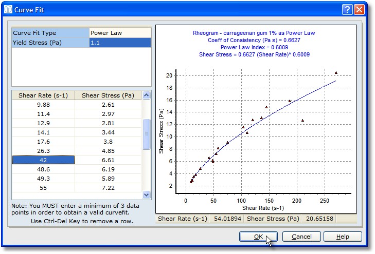
Power law modelling of rheology data

The example opposite shows viscometer data for a non-Newtonian fitted to a Power Law relationship.

FluidFlow3 uses different friction factor relationships for each available model, the relationships are valid over all flow regimes.

Heat Transfer Capabilities

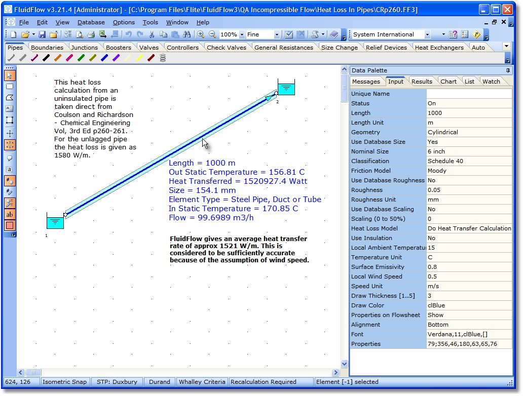
Pipe heat loss calculation

The example opposite shows the heat loss from a 1 kilometer length of uninsulated pipe.

There are over 300 QA example calculations made before each release of FluidFlow3. This is one of the verification heat transfer calculation examples.

A loss of 1520 kW over the pipe length represents energy wastage of over 1 million dollars per year.

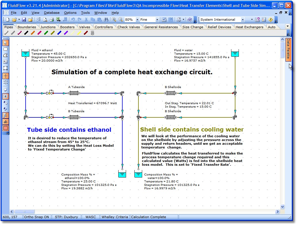
Heat Exchanger Modelling

An example circuit showing 2 heat exchangers with full modelling of both the shell and tubeside. Usually modelling of one side is sufficient.

Several Pressure Loss correlations can be used including: Deleware method, using manufacturers loss data, or using a fixed pressure loss.

With the 2-phase module you can also consider condensors and evaporators.

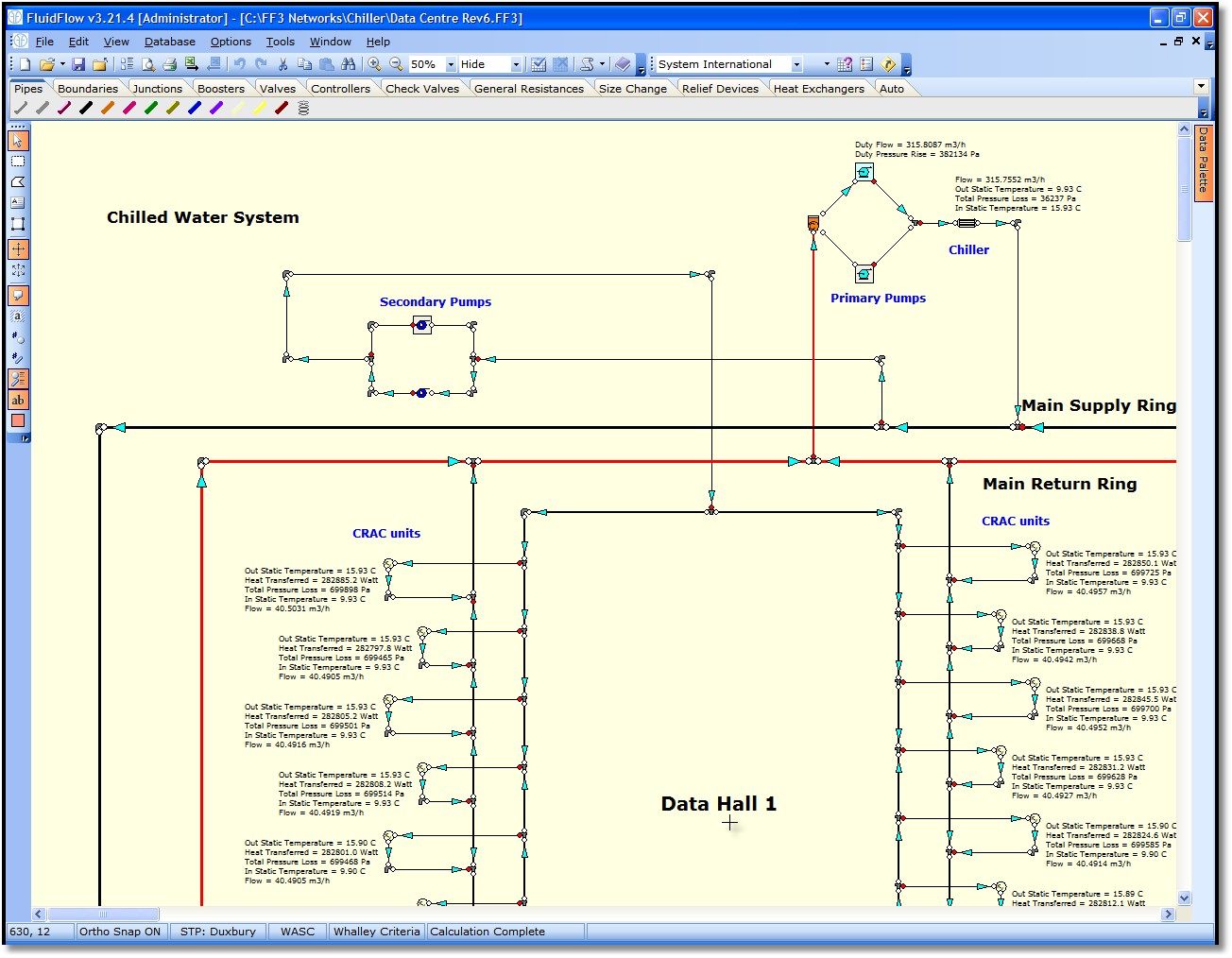
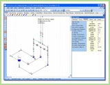
Larger network showing the design of a computer data centre

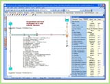
This network, shows how FluidFlow3 is used by a customer to model a chilled water cooling system in a Data Centre. Modelling of what happens due to pump failures is also considered in this model.

We have many other customers who model chiller circuits and/or district heating circuits using FluidFlow3.

One customer has sucessfully modelled the chiller system for Heathrow Airport and another the storage tank heating system at Europoort. Both networks contain over 5000 pipes and node and solve in a few minutes.

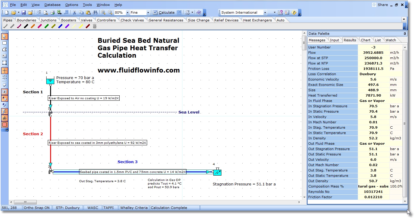
Buried Pipe Heat Transfer Calculation

In this example system, we have an offshore natural gas production platform exporting gas at 80°C via a 100km, 20" buried sea-bed pipeline. The pipeline is modelled in three sections as follows:

• Pipe segment exposed to air (no coating).
• Pipe segment exposed to sea coated in 3mm polyethylene.
• Pipe segment running along the sea bed coated with 1.5mm PVC and 75mm concrete.

The overall heat transfer coefficients for each pipe segment have been established from the table of typical values. The air and sea temperatures used in the example are 10°C and 5°C degrees respectively.

This heat transfer example is one of many FluidFlow3 verification examples and the calculated results have been compared to those available from the software package known as "Gas/dp" which is discontinued. Note, the results produced by the "Gas/dp" program were in the past widely accepted as having a relatively high degree of accuracy.

A PDF summary of the calculated results is available by clicking: "Sea Bed Model Datasheet".

Dynamic Analysis & Scripting

Control Valve Turndown [1m 32s]

Scripting allows you to change any property of any network element and then watch the response of any other property. In this example we change the speed of a pump and watch how flow control valves respond as well as watching the pump duty point adjust on the pump performance chart.

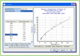
Pump Optimisation [40s]

In this example we will find the optimum pump operating speed if we run 5 pumps in parallel. The optimium speed depends on the number of pumps operating and can be markedly different.

We will run a script that asks how many pumps we wish to run. The script solves the system for a series of pump speeds ranging from the minimum to maximum operating speed. Results are exported to Excel (Flow, Speed, and Power needed per kg of fluid pumped).

Finally, the script plots an excel chart, so we can see easily where the optimum speed lies.